Intro to Online Learning

(Based on the Online Learning Course @ PoliMI (2022) by Francesco Trovò)

Intro

The general framework is the same as standard non-stationary learning, which means

• the environment is changing or even adversarial
• it is needed to both learn and adapt

In such a setting, each time instant

1. we generate a prediction $\hat y_t$ (with a model $\mathcal M$ or without)
2. the environment on the other hand generates $y_t$
3. a loss $l(\hat y_t, y_t)$ is suffered due to sum prediction error
4. a feedback $x_t$ might get returned
5. the model $\mathcal M$ (or whatever object we use for prediction) is updated accordingly to points 3 and 4

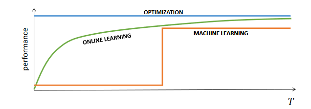
In order to gain good performances, it is required to balance between using all of the data stacks and being data efficient, that is making a sufficiently good prediction as soon as possible. Usually, a prediction corresponds to taking an action or performing a decision as well.

There are many different instances of online learning, the main idea is that the steps in Online Learning approaches are

1. For a specific problem setting: compute upper bounds (UB) and lower bounds (LB)
2. Design an algorithm $\mathcal A$
3. Check how much $\mathcal A$ fits the bounds (they should be the same in the best case)

Learning with Experts

The expert learning set consists of choosing online between a set of experts in order to act as the best expert (option), and predict as the best predictor. It is crucial to understand the type of feedback the environment returns, which is defined in terms of to which extent the information for one action is informative for the non-decided actions. It needs to be informative for the selected action at least.

In expert learning, the information $x_t$ consists of all the losses for any possible choice

Differently from the classical machine learning framework, in the online learning setting it is true that

• it is not possible to ensure fully stochastic processes
• the expected performances cannot be measured
• training and testing cannot be distinguished clearly
• data come in a sequence (stream)

Differently from learning in non-stationary environments

• it is not required to maintain a statistical characterization of the process
• it does not start from an initial model but starts from scratch
• it provides strong theoretical results

For these reasons, usually online learning starts from simple models and it compares the online performance with a clairvoyant optimal choice among the ones in a given set.

Finally, differently from reinforcement learning

• online learning is more like a meta-approach, which can be used in Reinforcement Learning as well. In fact, some Reinforcement Learning algorithms are online learning algorithms (i.e. Q-learning)
• Some online learning algorithms have been developed for Reinforcement Learning settings (i.e. UCB1)
• While Reinforcement Learning has some statistical assumptions on rewards and kernels, online learning can handle also adversarial settings.

For this reason, a concept of regret is introduced, which is not a quantity to be computed, but a concept over which to construct guarantees:

Given an algorithm, $\mathcal A$ selecting a prediction $\hat y_t$ at round $t$ and an optimal algorithm $\mathcal A^$ with $y^_t$, the (static) regret over the time horizon $T$ is defined as

depending on the environment the best prediction can be either

• the best constant prediction $y_t^* = \min_y \sum l(y,y_t)$
• the best constant average prediction $y^* = \min_y \sum \mathbb E \; [l(y,y_t)]$

The objective is to obtain a regret which is sub-linear in the time horizon T (no-regret algorithm) ( asymptotically converging towards the optimal as a by-product)

Binary Prediction

Outcome space $Y= {0,1}$, decision space $D = {0,1}$, loss function $l(\hat y, y)$, the learner chooses $\hat y_t$ the environment chooses $y_t$ and the environment reveals its choice leading to a loss.

Having access to an expert set $N$ over which there is only one single perfect expert

The experts are considered with weighting importance $w_{i,t}$.

In this setting, the Halving algorithm (H)

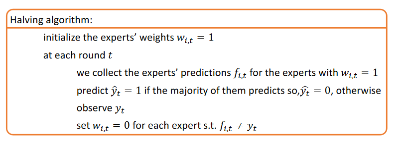
Theorem: following the Halving algorithm over a binary prediction problem with $N$ experts makes at most $m \leq \text{floor}(\log_2 N)$ mistakes if at least one expert is perfect.

Proof:

at each mistake (due to the majority of voters and breaking the tie at 50% with $\leq$):

In case there was no perfect expert it is not possible to discard all of them since it is not possible to know if they were still the best ones, it is just possible to shrink them by a factor of $\beta$, the proof follows when considering that one expert makes at most $m^*$ mistakes

If no expert is perfect, the objective is then to relate the number of mistakes made $m$ with the ones made by the best expert $m^*$ and this is done via a shrinking factor, the option is to use the Weighted Halving Algorithm (WHA)

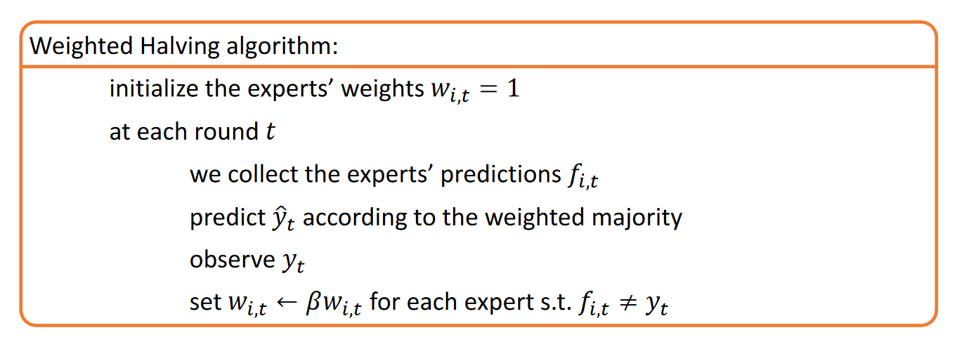
Theorem: following the WHA algorithm over a binary prediction problem with $N$ experts and a shrinking factor $\beta < 1$, makes at most $m \leq \text{floor}(\frac{\log_2 N - m^+\log_2\beta}{1-\log_2(1+\beta)})$ mistakes if at least one expert makes at most $m^*$ mistakes

Proof:

at each mistake, due to the majority of voters and breaking the tie at 50% with $\leq$

Since at least one expert makes at most $m^*$ mistakes

Convex Loss Prediction

Outcome space $Y$ arbitrary, decision space $D$ convex subset of $\mathbb R^s$, loss function $l(\hat y, y) \in [0,1]$ convex in the first argument (decision), the learner chooses $\hat y_t$ the environment chooses $y_t$ and the environment reveals its choice leading to a loss.

Consider any type of expert who might be

• fixed over time $f_{i,t} = c_i$
• adaptive to a context $f_{i,t} = f_i(x)$
• learning over past outcomes $f_{i,t} = f_i(t,y_1, \dots, y_{t-1})$
• adversarial

and a regret

since it is not possible to simply define mistakes.

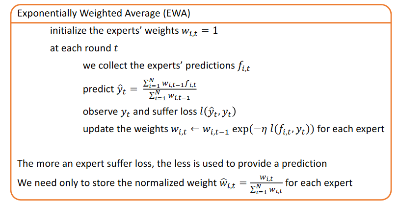
In such setting the algorithm which may be used is the Exponentially Weighted Average (EWA)

In order to prove this

Theorem: The EWA algorithm applied to continuous (convex) prediction problems with N experts and with parameter $\eta$ has regret

Proof:

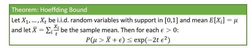
Remembering the Hoeffing inequality for a bounded random variable

Usually, once the regret bound is obtained, the best choice of the parameters are the ones that minimize or maximize such lower or upper bound, found by taking the derivative and setting it to $0$.

In the EWA case $\eta_n = \sqrt{\frac{8\log N}{n}}$, which has the problem of knowing the time-horizon $n$, which provides a regret

Such a result of EWA might be the best or not based on the properties of the loss functions, it is the best one for the bounded and convex or in the exp concave case, in other cases other algorithms might be better suited.

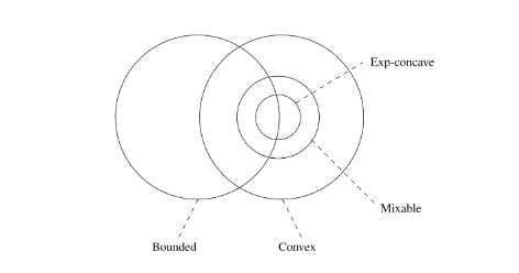
For example, the lower bound is different for

• Bounded and convex: $\Theta(n\log N)$ (matched by EWA)
• Mixable: $\Omega(\log N)$ (not necessarily matched by EWA)
• Exp Concave: $\Omega(n\log N)$

Convex Quadratic Prediction

In such cases, one idea is the Follow the Leader (FL)

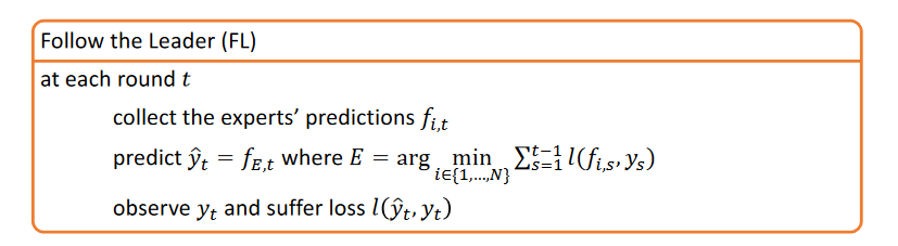
Theorem: The FL algorithm applied to a continuous prediction problem with constant experts and quadratic losses has regret

Other algorithms:

• Gradient-based EWA forecaster: gradient of the loss in the weight update
• Multilinear forecaster $w \leftarrow w(1+ \eta h(f,y))$
• Greedy forecaster: choose the expert who minimizes the worst case loss at the next step combined with its loss up to now
• Online Gradient Ascent: update the prediction in a single step in the direction of the gradient

Non-convex Loss Prediction

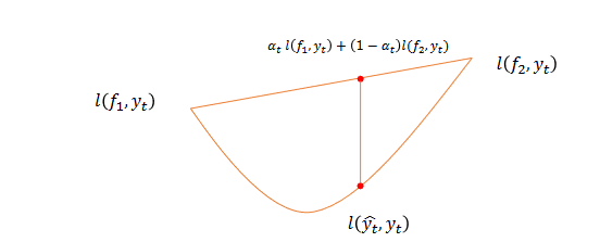
The convexity of the losses is required in order to be able to combine different experts while knowing that the combination will for sure lead to at least the same loss as one of them (it is always an overestimation)

It is not possible to use deterministic algorithms in such cases since the environment may always be able to give worst case prediction, leading to

The solution is then to use randomized algorithms over an equaivalent problem to the continuous non-convex one.

Outcome space $Y’ = Y \times D’^N$, decision space $D’ = {p \in [0,1]^N: \sum\pi_i = 1}$, experts $f’_{i,t} = (0, \dots, 1, \dots, 0) \in D$ with $1$ at i, loss function $l’(p,( y, f_1, \dots, f_n)) = \sum p_i l(f_i,y)$ convex (again) in the first argument.

Then in expectation we have a deterministic loss as in EWA by predicting with $I_t$ drawn from the distribution $\hat p_1, \dots, \hat p_N$

In such cases, the weights of EWA for example have to be used as probabilities, leading to the Randomized EWA (REWA).

Such an algorithm has the same bounds as the deterministic one but just in expectation so that one specific realization might be arbitrarily bad.

PAC Variation

In order to have a high probability bound (PAC) bound Hoeffding-Azuma-like inequalities for a set of $n$ bounded random variables

Applying it to $X_t = l(I_t, y_t)$ with $\delta$ being the righten side

Merging the PAC bound and the bounds in expectation we obtain that

Theorem: The REWA algorithm applied to a discrete prediction problem with N experts and with parameter $\eta = \sqrt{\frac{8\log N}{n}}$ satisfies with probability at least $1-\delta$

The same considerations go for FL, since it is a deterministic algorithm. It needs to be randomized with a random perturbation, leading to Follow the Perturbed Leader (FPL)

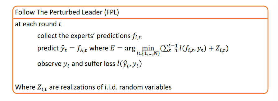
Theorem: The FPL algorithm applied to a discrete prediction problem with N experts satisfies

Thus the result is worse than REWA generally. The order of $\log N$ can be restored by tuning the random variables by using a two-sided exponential distribution $p(z) = (\frac{\eta}{2})^Ne^{-\eta\vert Z \vert}$ with $\eta >0$

Portfolio Optimization

Portfolio optimization scenarios are the ones where the outcome space $Y$ is discrete and the decision space $D = \Delta^N$,

• Given a budget $W_0$ you should invest over a set on $N$ different stocks
• At each time step, a distribution of the budget over the available stocks needs to be chosen $\hat y_t = (\hat y_{1,t}, \dots, \hat y_{N,t})$
• The environment chooses a vector of results telling the stock prices $y_t = (y_{1,t}, \dots, y_{N,t})$
• At the end of $n$ investments steps, the reward is

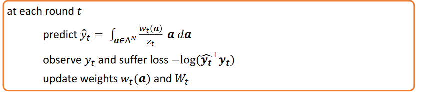
The loss can be seen as $l(\hat y_t, y_t) = - \log W_n = -\log W_0 - \sum^n \log (\hat y_t ^\top y_t)$

Then the (static) regret is

In this setting, a continuous version of EWA should be used (CEWA) where $w_t(a\in D) = \exp(-\eta \sum_t^{t-1}-\log(a^\top y_t), z_t = \int_a w_t(a)da$

Theorem: The CEWA algorithm applied to an online portfolio optimization problem with N stocks and with parameter $\eta = 2\sqrt{\frac{Nn\log n}{2}}$ has regret

which is sub-linear but can be improved by universal portfolio approaches.

Learning with Limited Feedback (MAB)

All of these settings are similar to a standard optimization with the main difference being that the regret is taken into account, meaning that the way the optimum is reached matters as well.

How to tackle such settings?

• Traditional ML? No, a dataset is not available at the beginning
• Expert Learning? No, the feedback is not full but limited to the action tried
• Adversarial Approaches? No, sometimes there is no adversarial out of ignorance (lack of information)
• Online Learning? Yes, the decision should be improved as soon as new data arrives

In the expert setting, the feedback was assumed to be informative about what would have happened in case some other action was selected. In case the feedback is related just to the selected actions (i.e. limited) then the framework is the so-called Multi-Armed Bandit.

The framework consists of a repeated game one with a finite horizon. This definition leads to the additional requirement compared to Expert Learning: a balance between exploiting the best-action so far and exploring new options, i.e. information gathering (exploration-exploitation dilemma).

In order to study the performance of my choices, a regret for an algorithm $A$ is defined as

Adversarial Setting

An interesting setting is the adversarial setting, where the rewards are chosen by an opponent who

• knows the algorithm
• chooses all the rewards in advance

In such a scenario, the (adversarial) (static) regret is defined against the best constant choice $i$ among the ones available, compared to the selected option $I_t \in {1, \dots , K}$, getting respectively a reward $g_{i,t}$ and $g_{I_t, t}$ (bounded for simplicity) (in a not adversarial setting the notation is $Y_{i,t}$)

where the expectation is taken with respect to the stochasticity of the algorithm.

Algorithms

The idea in such setting is to use a modified version of the REWA forecaster updating only the observed loss (or gain), since as in the expert setting the prediction space is discrete and finite and the loss is generic, leading to Exp3

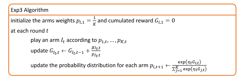
Theorem: The Exp3 algorithm applied to an adversarial MAB with $K$ arms and a parameter $\eta_n = \sqrt{\frac{2 \log K }{n K}}$ suffers a regret of

Notice that $\eta_n$requires knowing the horizon beforehand. Interestingly, with respect to the expert case, the regret worsen to a $K \log K$ with respect to $\log K$, due to less information.

If $\eta_t = \sqrt{\frac{\log N}{tk}}$ is used, not depending on $n$ but changing over time, the regret becomes

Yet, both hold in expectation, and for this reason, this is usually called pseudo-regret.

Lower Bound

Actually it is not possible to improve more than the $\sqrt K$ term since the lower bound is given by

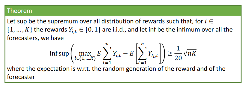
This min-max lower bound is given in the generic, not adversarial setting, and as such is more general.

PAC Variation

In case the results are required to hold in high probability (PAC), concentration inequalities have to be used. This leads to the Exp3.P algorithm

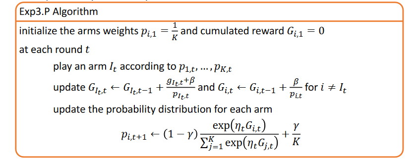
where the $\gamma$ factor guarantees small exploration even under no rewards at all, the same goes for $\beta$. For this algorithm

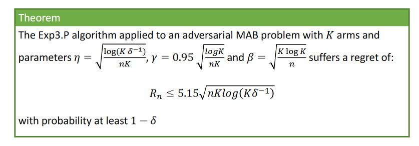
noting that having a result in high-probability $1-\delta$ it is always possible to study it in expectation by

Stochastic (stationary) Setting

In the Stochastic MAB setting there is a double source of stochasticity both due to the algorithm and the reward which is sampled according to a distribution. This is the case for slot machines, game playing, advertisements, and clinical trials. This setting is a specific case of an MDP $(S,A,P,R,\gamma,\mu_0)$ with a single state, $A$ the set of arms $D$ ($I_t$ is selected according to a policy whose support is $D$) and a trivial kernel, thus any strategy for solving sample-based MDPs (RL) is also a strategy to solve MAB, even though RL does not usually have regret bounds.

In this setting, stochastic regret can be defined with respect to expected rewards $\mu_i = \mathbb E[Y_{i,t}]$

where the expectation is with respect to the forecaster’s stochasticity. This regret can be rewritten with $\Delta_i = \mu^* - \mu_i$ and $N_{i,t}$ the number o times the arm $i$ was selected

Lower Bound

In such cases, it holds a lower bound

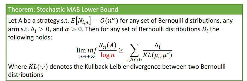
usually $KL \propto \Delta^2$ so the constant which multiplies $\log n$ scales with $\frac{1}{\Delta_i}$: the more the arms are similar to the optimal arm, the longer it will take to distinguish the optimal one.

Note that by setting $\alpha=0$ there would be a small probability to fail but still an infinite time to regret it.

Algorithms

A first algorithm for Stochastic MABs is the greedy algorithm

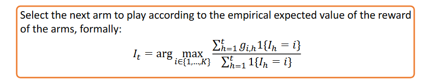
with this algorithm the regret is given by

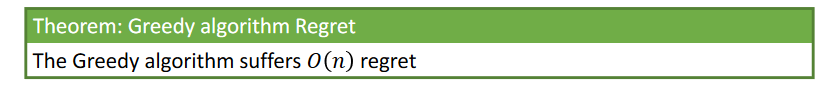
where the worst case is when with Bernoulli distributions the first time the optimal arm is pulled a $0$ reward is returned, thus the optimal arm will never be pulled again. The probability of this happening is a low constant but non-zero, then bounding the whole regret.

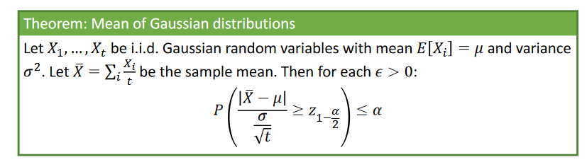
Another approach is then to use optimism in the face of uncertainty, by using some concentration inequalities such as for the Gaussians

or for sub-gaussians

By using these, the objective is to define an $\epsilon$ that is able to minimize such quantity. Then, instead of selecting the arm with the largest sample mean $\bar Y_{i,t}$, an optimistic estimator of the expected value is usedù

In the MAB case

leading to

therefore the objective is to have a limited amount of mistakes for each arm for each possible number of pulls

by selecting $p(t) = 1/t^4$, $b_{i,t} = \sqrt{\frac{2\log t}{N_{i,t}}}$, leading to UCB1

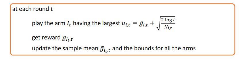
with a regret bound

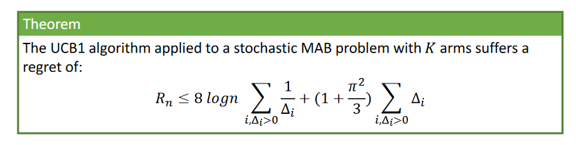
This bound is distribution dependent, and up to a constant it matches the lower bound, so it is the one of an optimal algorithm. In general, it might be possible to improve over the LB on specific MABs and on specific runs might get null regret as well (regret in expectation).

Bayesian Approach

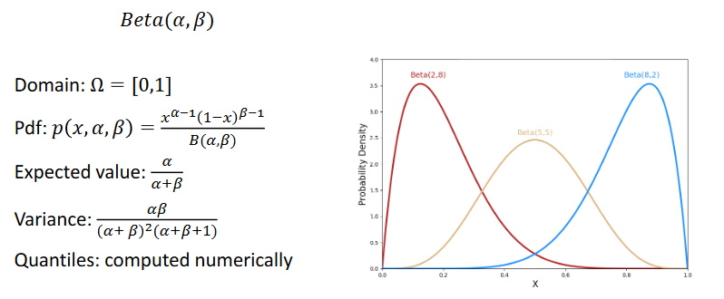
Instead of estimating the expected reward as the empirical mean, distribution is used. Such distribution is updated by Bayesian rule over conjugate prior/posterior tricks, which guarantee to have incremental algorithms, as for

• Gaussian/Gaussian (known variance)
• Gamma/Gaussian (known mean)
• Beta/Bernoulli

The prior/posterior trick comes from the fact that for example updating a Beta with a sample coming with a Bernoulli the result of a Bayes update will be again a Beta.

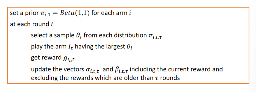
An example of such methods is Thompson Sampling (TS)

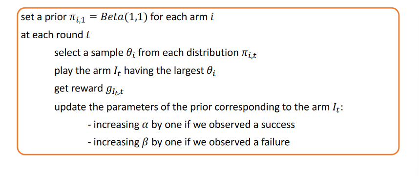
which shows regret with matching upper-bound

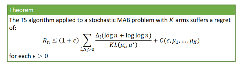
Beyond Stochasticity

Contextual MAB

In these settings there exist side information $\theta$ that can be used to infer. In case some structure is present in the reward function novel methods can be used, otherwise, we are solving a MAB for each context.

In the linear contextual case, $Y_t = X_t^\top\theta + \eta_t$ for each given arm $X_t \in \mathbb R^d$, a context $\theta$ (in linear correlation with the selected arm) and some noise $\eta_t$. In such cases for instance one idea might be to compute the best possible estimates of the context and then add a bound holding for all the $d$ dimensions.

Fon non-linear contextual cases, Gaussian Process Kernels might be used to estimate the context, leading to GP-UCB and GP-TS.

Cops and Robbers

This instance has special feedback since the learner observes the losses associated with all actions except the played action. Except for constant factors, this problem is no harder than the full information setting where all losses are observed, in fact the regret can be upper bounded by

Stochastic (non-stationary) Setting

In such a setting, the expected value of the rewards might change over time

• In a abrupt way: meaning that there exist a set of phases $\phi = {b_0, \dots, b_\Gamma}$ in the learning process identified by some breakpoints, over which the rewards have constant expected value
• In a smooth way: the expected reward of each arm has some regularity though, as for lipschitzianity over time.

The static regret is not informative in these settings and a stochastic dynamic regret is introduced as

Abrupt Changing

Two different approaches are possible

• Passive larning: it does not try to detect the breakpoints but it rather uses more information of the near past over a predefined time window
• Active learning: it uses a CDT to decide when the breakpoints occurred

In the first case, one example is the SW-UCB algorithm

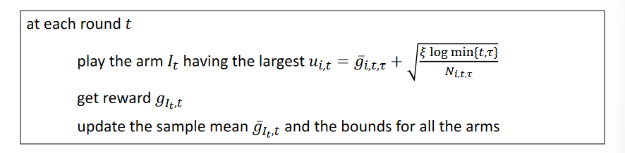
with dimensions defined over the last $\tau$ rounds. This algorithm has a regret of

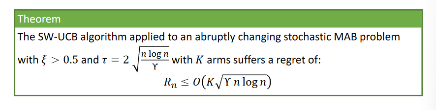
Nonetheless, this regret requires to know the number of breakpoints $\Gamma$ and the horizon $n$ and finally it does not actually scale well with it.

In the second case, standard MAB algorithms might be used in parallel to standard CDT algorithms, yet the issue here is that they receive samples from an arm according to its performance. This means that for each round $t$

• The suboptimal amrs are pulled $O(\log t / \Delta_{i,t})$ times
• The optimal arm is pulled $O(t)$ times

Therefore the expected delay in the detection is of the order of the inverse of the suboptimal case.

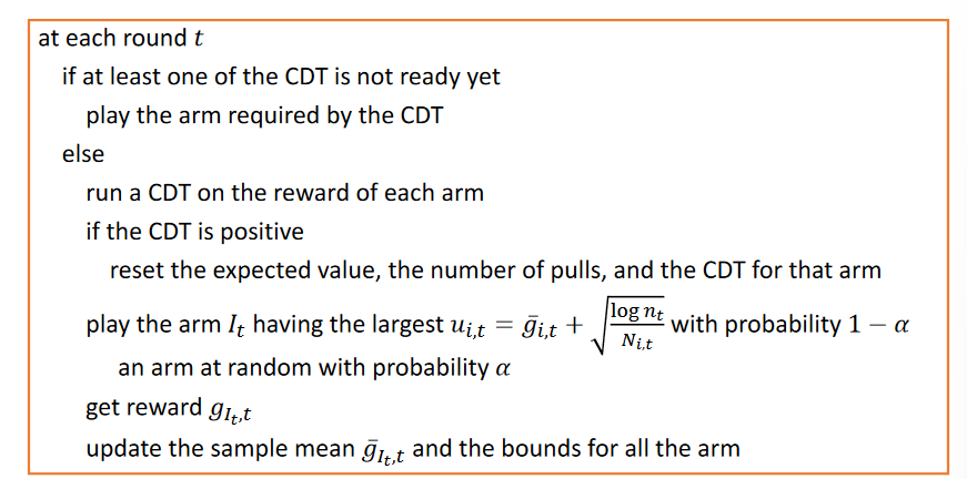
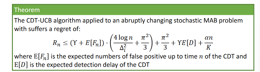
One proposed approach is the CDT-UCB algorithm:

with a regret given by

Active methods have advantages and disadvantages, respectively

• Pros: they are able to directly identify the change and in general they are more powerful than passive approaches
• Cons: they require more knowledge over the problem

Smooth Changing

Under the assumptions that the number of times arms are closer than $\Delta$ over the time horizon is bounded by $H(\Delta,n) \leq F\Delta T$ and that the Lipschitz constant for the variation of the mean reward is $\sigma$, the first algorithm is SW-KL-UCB:

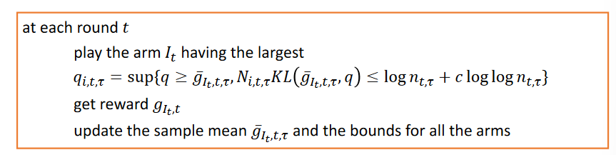
which suffers a regret given by

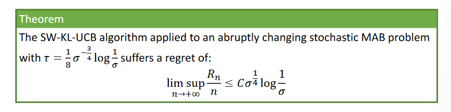
which is not vanishing but limited per-round by $\sigma$.

Both changes

The idea is given by Trovò, F., et al. “Sliding-Window Thompson Sampling for Non-Stationary Settings.” JAIR 2020

which suffers a regret given by